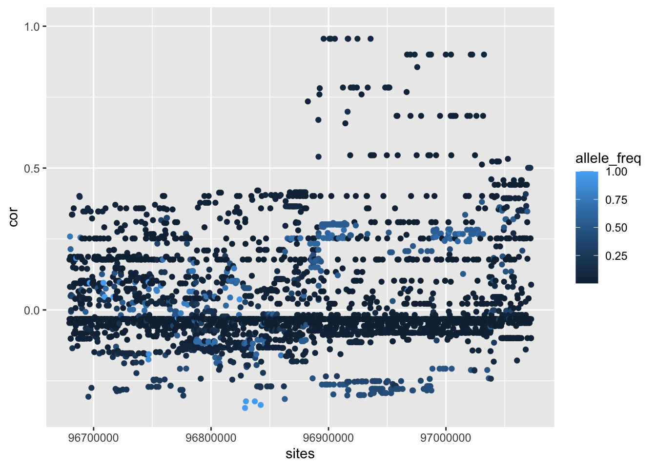
analyzing-ERAP2-personalized-mutagenesis

Author

Saideep Gona

Published

April 4, 2023

Code

suppressMessages(library(tidyverse))
suppressMessages(library(glue))
PRE = "/Users/saideepgona/Library/CloudStorage/Box-Box/imlab-data/data-Github/Daily-Blog-Sai"

## COPY THE DATE AND SLUG fields FROM THE HEADER
SLUG="analyzing-ERAP2-personalized-mutagenesis" ## copy the slug from the header
bDATE='2023-04-04' ## copy the date from the blog's header here
DATA = glue("{PRE}/{bDATE}-{SLUG}")
if(!file.exists(DATA)) system(glue::glue("mkdir {DATA}"))
WORK=DATA

#TODO

Context

It’s time to analyze the ERAP2 mutagenesis results from reference-based and individual mutagenesis

Load in relevant metadata

Code

metadata_dir = "/Users/saideepgona/Library/CloudStorage/Box-Box/imlab-data/data-Github/analysis-Sai/metadata"

pop_metadata <- read_delim(file.path(metadata_dir,"relationships_w_pops.txt"))
rownames(pop_metadata) <- pop_metadata$IID

gene_annotations <- read_csv(file.path(metadata_dir,"ref_local_ancestry","gene_annotations.csv"))
genes <- as.vector(gene_annotations$...1)
gene_annotations <- gene_annotations[,2:ncol(gene_annotations)]
rownames(gene_annotations) <- genes

gene_annotations["ENSG00000164308",]

# A tibble: 1 × 6
    AFR   AMR   EAS   SAS   EUR  `NA`
  <dbl> <dbl> <dbl> <dbl> <dbl> <dbl>
1     0     0     0     0     0 43717

Code

sum(rowSums(gene_annotations)==0)

[1] 11

Code

hist(rowSums(gene_annotations))

Code

# Geuvadis expression
dset_dir <- "/Users/saideepgona/Library/CloudStorage/Box-Box/imlab-data/data-Github/analysis-Sai/enformer_geuvadis/enformer_portability_analysis"
geuvadis_full <- read_delim(file.path(dset_dir,"GD462.GeneQuantRPKM.50FN.samplename.resk10.txt"))
geuvadis_genes_symbols <- sapply(str_split(geuvadis_full$Gene_Symbol, "\\."),`[`,1)
geuvadis <- as.data.frame(geuvadis_full[,5:ncol(geuvadis_full)])
rownames(geuvadis) <- geuvadis_genes_symbols

Code

data_dir = "/Users/saideepgona/Library/CloudStorage/Box-Box/imlab-data/data-Github/analysis-Sai/enformer_geuvadis/ERAP2_personalized_mutagenesis"

genotype_data <- read_csv(file.path(data_dir,"genotypes_df.csv"))
variant_ids <- as.vector(genotype_data[,1])[[1]]
rownames(genotype_data) <- as.vector(genotype_data[,1])[[1]]

genotype_data[,1] <- NULL
rownames(genotype_data) <- variant_ids

allele_count_df <- ifelse(genotype_data=="1|1",2,ifelse(genotype_data=="0|0",0,1))
rownames(allele_count_df) <- variant_ids

variant_metadata_df <- data.frame(af=rowSums(allele_count_df)/(2*ncol(allele_count_df*2)))

Effect size of reference variants alone

It will help to have the effect size of these variants when using a reference background alone. We can load these in:

Code

data_dir = "/Users/saideepgona/Library/CloudStorage/Box-Box/imlab-data/data-Github/analysis-Sai/enformer_geuvadis/ERAP2_personalized_mutagenesis"

haplo1_ref <- read_csv(file.path(data_dir,"erap2_personalized_LCL_REF_quantification_haplo1.csv"))
haplo1_ref <- haplo1_ref[,3:ncol(haplo1_ref)]

haplo1_ref_rc <- read_csv(file.path(data_dir,"erap2_personalized_LCL_REF_quantification_haplo1_rc.csv"))
haplo1_ref_rc<- haplo1_ref_rc[,3:ncol(haplo1_ref_rc)]

haplo1_ref_ave = data.frame(t((haplo1_ref_rc + haplo1_ref)/2))
colnames(haplo1_ref_ave) <- c("expression")

reference_hap_expression <- as.numeric(haplo1_ref_ave[1,1])


haplo2_ref <- read_csv(file.path(data_dir,"erap2_personalized_LCL_REF_quantification_haplo2.csv"))
haplo2_ref <- haplo2_ref[,3:ncol(haplo2_ref)]

haplo2_ref_rc <- read_csv(file.path(data_dir,"erap2_personalized_LCL_REF_quantification_haplo2_rc.csv"))
haplo2_ref_rc <- haplo2_ref_rc[,3:ncol(haplo2_ref_rc)]

haplo2_ref_ave = data.frame(t((haplo2_ref_rc + haplo2_ref)/2))
colnames(haplo2_ref_ave) <- c("expression")

Code

ref_dif <- haplo2_ref_ave - haplo1_ref_ave
colnames(ref_dif) <- c("dif")

ref_dif$ids <- rownames(ref_dif)
ref_dif <- ref_dif %>% separate(ids,into = c("individual","mutated_variant","ref"))

ref_dif$pos <- as.numeric(ref_dif$mutated_variant)

ref_dif$voi <- ifelse(ref_dif$mutated_variant %in% c("96916885","96916728","96900192"),TRUE,FALSE)
ref_dif$voi_sizes <- as.numeric(ifelse(ref_dif$mutated_variant %in% c("96916885","96916728","96900192"),15,1))

ref_dif$allele_freq <- as.numeric(variant_metadata_df[ref_dif$mutated_variant,1])

Code

ggplot(ref_dif) + geom_point(aes(x=pos,y=dif, color = allele_freq), alpha=0.5) + scale_x_continuous(breaks = seq(96875986-80000, 96875986+80000, by = 20000)) + theme(axis.text.x = element_text(angle = 90, vjust = 0.5, hjust=1)) + geom_vline(xintercept = 96875986) + ylab("variant effect magnitude") + xlab("position on chr5") + ggtitle("In-silico mutagenesis of ERAP2 variants")

Code

ggplot(ref_dif) + geom_point(aes(x=allele_freq, y=dif))

Ok, let’s see how well some of these interesting variants correlate with the expression patterns we are seeing:

Calculate true individual-specific expression estimates, this first requires loading the personalized expression:

Code

library(tidyverse)

haplo1 <- read_csv(file.path(data_dir,"erap2_personalized_LCL_quantification_haplo1.csv"))
haplo1 <- haplo1[,3:ncol(haplo1)]

haplo1_rc <- read_csv(file.path(data_dir,"erap2_personalized_LCL_quantification_haplo1_rc.csv"))
haplo1_rc<- haplo1_rc[,3:ncol(haplo1_rc)]

haplo1_ave = data.frame(t((haplo1_rc + haplo1)/2))
colnames(haplo1_ave) <- c("expression")


haplo2 <- read_csv(file.path(data_dir,"erap2_personalized_LCL_quantification_haplo2.csv"))
haplo2 <- haplo2[,3:ncol(haplo2)]

haplo2_rc <- read_csv(file.path(data_dir,"erap2_personalized_LCL_quantification_haplo2_rc.csv"))
haplo2_rc <- haplo2_rc[,3:ncol(haplo2_rc)]

haplo2_ave = data.frame(t((haplo2_rc + haplo2)/2))
colnames(haplo2_ave) <- c("expression")

Code

haplo1_ave$ids <- rownames(haplo1_ave)
haplo1_ave <- haplo1_ave %>% separate(ids,into = c("individual","mutated_variant","mutated_genotype"))
haplo1_ave$haplotype <- "1"

haplo1_ref <- haplo1_ave[haplo1_ave$mutated_genotype == "REF",]
haplo1_alt <- haplo1_ave[haplo1_ave$mutated_genotype == "ALT",]

haplo2_ave$ids <- rownames(haplo2_ave)
haplo2_ave <- haplo2_ave %>% separate(ids,into = c("individual","mutated_variant","mutated_genotype"))
haplo2_ave$haplotype <- "2"

haplo2_ref <- haplo2_ave[haplo2_ave$mutated_genotype == "REF",]
haplo2_alt <- haplo2_ave[haplo2_ave$mutated_genotype == "ALT",]

ref_stack <- rbind(haplo1_ref,haplo2_ref)
alt_stack <- rbind(haplo1_alt,haplo2_alt)

full_df <- data.frame(individual=ref_stack$individual,haplotype=ref_stack$haplotype,mutated_variant=ref_stack$mutated_variant, ref_expression=ref_stack$expression, alt_expression=alt_stack$expression)

Code

erap2_expression <- c()
  
for (ind in colnames(genotype_data)) {
  expression = 0
  cur_geno = str_split(genotype_data["96916885",ind], "|")
  
  if (cur_geno[[1]][2] == "0") {
    id_tag = paste(ind,"96916885","REF", sep="_")
    expression = expression + haplo1_ave[id_tag,]$expression
  } else {
    id_tag = paste(ind,"96916885","ALT", sep="_")
    expression = expression + haplo1_ave[id_tag,]$expression
  }

  if (cur_geno[[1]][4] == "0") {
    id_tag = paste(ind,"96916885","REF", sep="_")
    expression = expression + haplo2_ave[id_tag,]$expression
  } else {
    id_tag = paste(ind,"96916885","ALT", sep="_")
    expression = expression + haplo2_ave[id_tag,]$expression
  }
  
  erap2_expression <- c(erap2_expression, expression)
}

Let’s also grab the large effect size variants from the reference mutagenesis:

Code

ref_dif[ref_dif$dif > 4,]

                            dif individual mutated_variant ref      pos   voi
reference_96876409_REF 5.024243  reference        96876409 REF 96876409 FALSE
reference_96896518_REF 9.473810  reference        96896518 REF 96896518 FALSE
                       voi_sizes allele_freq
reference_96876409_REF         1   0.0200000
reference_96896518_REF         1   0.5628571

Code

erap2_expression_df <- data.frame(enformer_predicted_whole_expression=erap2_expression,
                                  geuvadis_expression = as.numeric(geuvadis["ENSG00000164308",colnames(genotype_data)]),
                                  fm_96916885_geno=allele_count_df["96916885",],
                                  splice_96900192_geno=allele_count_df["96900192",],
                                  fm_96916728_geno=allele_count_df["96916728",],
                                  large5_96876409_geno=allele_count_df["96876409",],
                                  large10_96896518_geno=allele_count_df["96896518",])
rownames(erap2_expression_df) <- colnames(genotype_data)

erap2_expression_df$ancestry <- as.vector(pop_metadata[rownames(erap2_expression_df),]$population)

ggplot(erap2_expression_df) + geom_point(aes(x=geuvadis_expression, y=enformer_predicted_whole_expression, color=ancestry)) + xlab("Geuvadis Expression for ERAP2") + ylab("Enformer predicted ERAP2 expression") + ggtitle("Predicted vs. Observed ERAP2 expression across individuals")

Code

ggplot(erap2_expression_df) + geom_point(aes(x=geuvadis_expression, y=enformer_predicted_whole_expression, color=splice_96900192_geno, shape=ancestry))

Code

ggplot(erap2_expression_df) + geom_point(aes(x=geuvadis_expression, y=enformer_predicted_whole_expression, color=fm_96916885_geno, shape=ancestry))

Code

ggplot(erap2_expression_df) + geom_point(aes(x=geuvadis_expression, y=enformer_predicted_whole_expression, color=fm_96916728_geno, shape=ancestry))

Code

ggplot(erap2_expression_df) + geom_point(aes(x=geuvadis_expression, y=enformer_predicted_whole_expression, color=large5_96876409_geno, shape=ancestry))

Code

ggplot(erap2_expression_df) + geom_point(aes(x=geuvadis_expression, y=enformer_predicted_whole_expression, color=large10_96896518_geno, shape=ancestry))

Let’s generate predicted personalized gene expression by summing up individual variant effects with the reference prediction as a baseline:

Code

allele_count_mat <- as.data.frame(allele_count_df)

dif_mat <- data.frame(difs = ref_dif$dif)
rownames(dif_mat) <- ref_dif$mutated_variant

allele_count_mat <- t(as.matrix(allele_count_mat[rownames(dif_mat),]))
dif_mat <- as.matrix(dif_mat)

linear_predictions <- allele_count_mat %*% dif_mat + reference_hap_expression*2

erap2_expression_df$linear_pred <- as.vector(linear_predictions)

ggplot(erap2_expression_df) + geom_point(aes(x=linear_predictions, y= enformer_predicted_whole_expression, color=ancestry)) + ylab("Enformer predicted ERAP2 expression") + xlab("Sum of variant effects") + ggtitle("Enformer predicted ERAP2 expression vs. sum of individual Enformer variant \n effects for ERAP2")

The above plot plots the individualized expression predictions

Clearly, ERAP2 is well predicted as a linear sum of individual variant effects. This supports the conclusion that the large effect variant is at play here.

personalized mutagenesis

After loading in the personalized expression estimates

We can also annotate each value with data for the individual, haplotype, mutated variant, and genotype of mutated variant.

Code

library(tidyverse)

haplo1 <- read_csv(file.path(data_dir,"erap2_personalized_LCL_quantification_haplo1.csv"))
haplo1 <- haplo1[,3:ncol(haplo1)]

haplo1_rc <- read_csv(file.path(data_dir,"erap2_personalized_LCL_quantification_haplo1_rc.csv"))
haplo1_rc<- haplo1_rc[,3:ncol(haplo1_rc)]

haplo1_ave = data.frame(t((haplo1_rc + haplo1)/2))
colnames(haplo1_ave) <- c("expression")


haplo2 <- read_csv(file.path(data_dir,"erap2_personalized_LCL_quantification_haplo2.csv"))
haplo2 <- haplo2[,3:ncol(haplo2)]

haplo2_rc <- read_csv(file.path(data_dir,"erap2_personalized_LCL_quantification_haplo2_rc.csv"))
haplo2_rc <- haplo2_rc[,3:ncol(haplo2_rc)]

haplo2_ave = data.frame(t((haplo2_rc + haplo2)/2))
colnames(haplo2_ave) <- c("expression")

Code

haplo1_ave$ids <- rownames(haplo1_ave)
haplo1_ave <- haplo1_ave %>% separate(ids,into = c("individual","mutated_variant","mutated_genotype"))
haplo1_ave$haplotype <- "1"

haplo1_ref <- haplo1_ave[haplo1_ave$mutated_genotype == "REF",]
haplo1_alt <- haplo1_ave[haplo1_ave$mutated_genotype == "ALT",]

haplo2_ave$ids <- rownames(haplo2_ave)
haplo2_ave <- haplo2_ave %>% separate(ids,into = c("individual","mutated_variant","mutated_genotype"))
haplo2_ave$haplotype <- "2"

haplo2_ref <- haplo2_ave[haplo2_ave$mutated_genotype == "REF",]
haplo2_alt <- haplo2_ave[haplo2_ave$mutated_genotype == "ALT",]

ref_stack <- rbind(haplo1_ref,haplo2_ref)
alt_stack <- rbind(haplo1_alt,haplo2_alt)

full_df <- data.frame(individual=ref_stack$individual,haplotype=ref_stack$haplotype,mutated_variant=ref_stack$mutated_variant, ref_expression=ref_stack$expression, alt_expression=alt_stack$expression)

We now have collected all our estimates into a concise data frame. Next we can calculate some effect-size related estimates by comparing the alt,ref

Code

full_df$dif <- full_df$alt_expression-full_df$ref_expression
full_df$fc <- full_df$alt_expression/full_df$ref_expression
full_df$logfc <- log2(full_df$fc)

full_df$log_ref <- log(full_df$ref_expression)
full_df$log_alt <- log(full_df$alt_expression)

We can also annotate our results by individual ancestry

Code

full_df$ancestry <- as.vector(pop_metadata[full_df$individual,]$population)

Code

# TODO Plot against allele frequency
# TODO Color by ancestry 

ggplot(full_df) + geom_violin(aes(x=mutated_variant, y=dif, fill=mutated_variant)) + geom_jitter(aes(x=mutated_variant, y=dif))+geom_hline(yintercept = ref_dif[ref_dif$mutated_variant=="96916885","dif"], color="blue") + geom_hline(yintercept = ref_dif[ref_dif$mutated_variant=="96916728","dif"], color="green") + geom_hline(yintercept = ref_dif[ref_dif$mutated_variant=="96900192","dif"], color="red") +scale_color_manual(name='Personalized vs. ref mutagenesis',
                     breaks=c('96916885', '96916728', '96900192'),
                     values=c('96916885'='red', '96916728'='blue', '96900192'='green')) + theme(legend.title=element_text(size=20),
       legend.text=element_text(size=14))

Code

ggplot(full_df) + geom_violin(aes(x=mutated_variant, y=dif, fill=haplotype))

Code

ggplot(full_df) + geom_violin(aes(x=mutated_variant, y=dif, fill=ancestry))

The distributions are certainly interesting.

It would be good to try and identify if the 96916728 “positive” group is an interaction with a specific variant present more frequently in that subgroup.

Code

full_df_fm_96916728_pos <- full_df[(full_df$dif > 0) & (full_df$mutated_variant == 96916728),]

fm_96916728_pos_individuals <- unique(full_df_fm_96916728_pos$individual)


allele_count_sub <- as.data.frame(t(allele_count_df[rownames(dif_mat),]))

allele_count_sub$fm_96916728_pos <- rownames(allele_count_sub) %in% fm_96916728_pos_individuals

fm_96916728_pos_cor <- as.data.frame(cor(allele_count_sub[,colnames(allele_count_sub != "fm_96916728_pos")],allele_count_sub$fm_96916728_pos))

fm_96916728_pos_cor$sites <- as.numeric(rownames(fm_96916728_pos_cor))
colnames(fm_96916728_pos_cor) <- c("cor", "sites")

fm_96916728_pos_cor$allele_freq <- as.numeric(variant_metadata_df[rownames(fm_96916728_pos_cor),1])

ggplot(fm_96916728_pos_cor) + geom_point(aes(x=sites,y=cor, col=allele_freq))