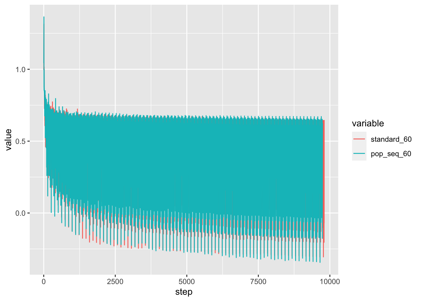
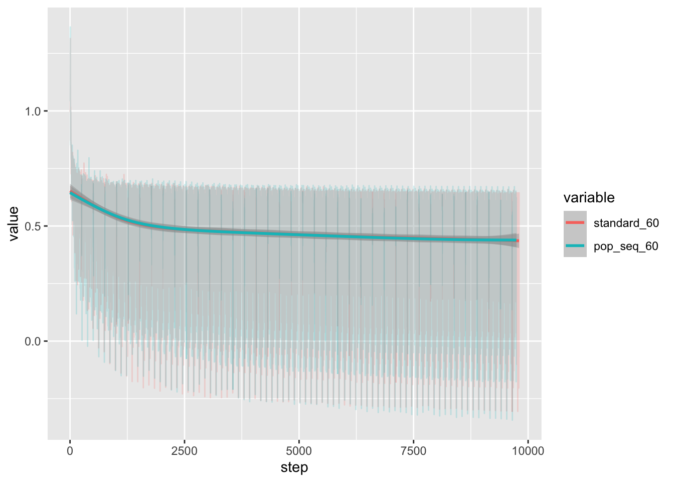
suppressMessages(library(tidyverse))suppressMessages(library(glue))PRE ="/Users/saideepgona/Library/CloudStorage/Box-Box/imlab-data/data-Github/Daily-Blog-Sai"## COPY THE DATE AND SLUG fields FROM THE HEADERSLUG="test_pop_seq_training"## copy the slug from the headerbDATE='2023-06-26'## copy the date from the blog's header hereDATA =glue("{PRE}/{bDATE}-{SLUG}")if(!file.exists(DATA)) system(glue::glue("mkdir {DATA}"))WORK=DATA
Context
Have been busy working on my thesis proposal, so couldn’t focus on interpreting the results of comparing the pop-seq with the standard sequences from the hackathon. Here I will begin that task
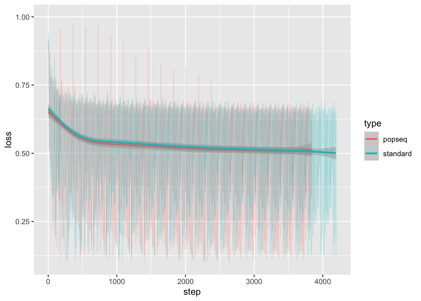
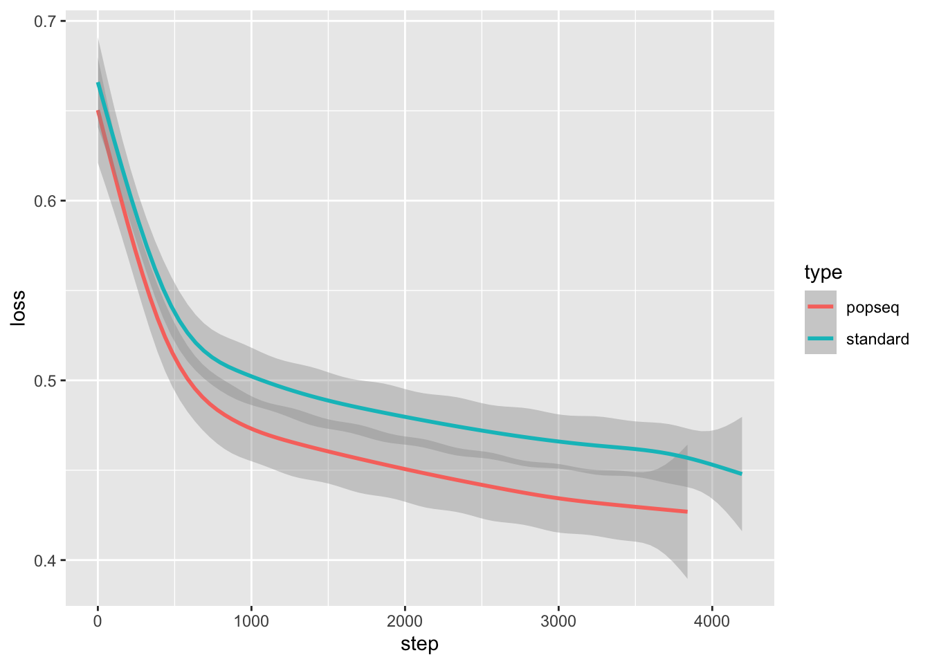
Comparing loss curves between the two training sets
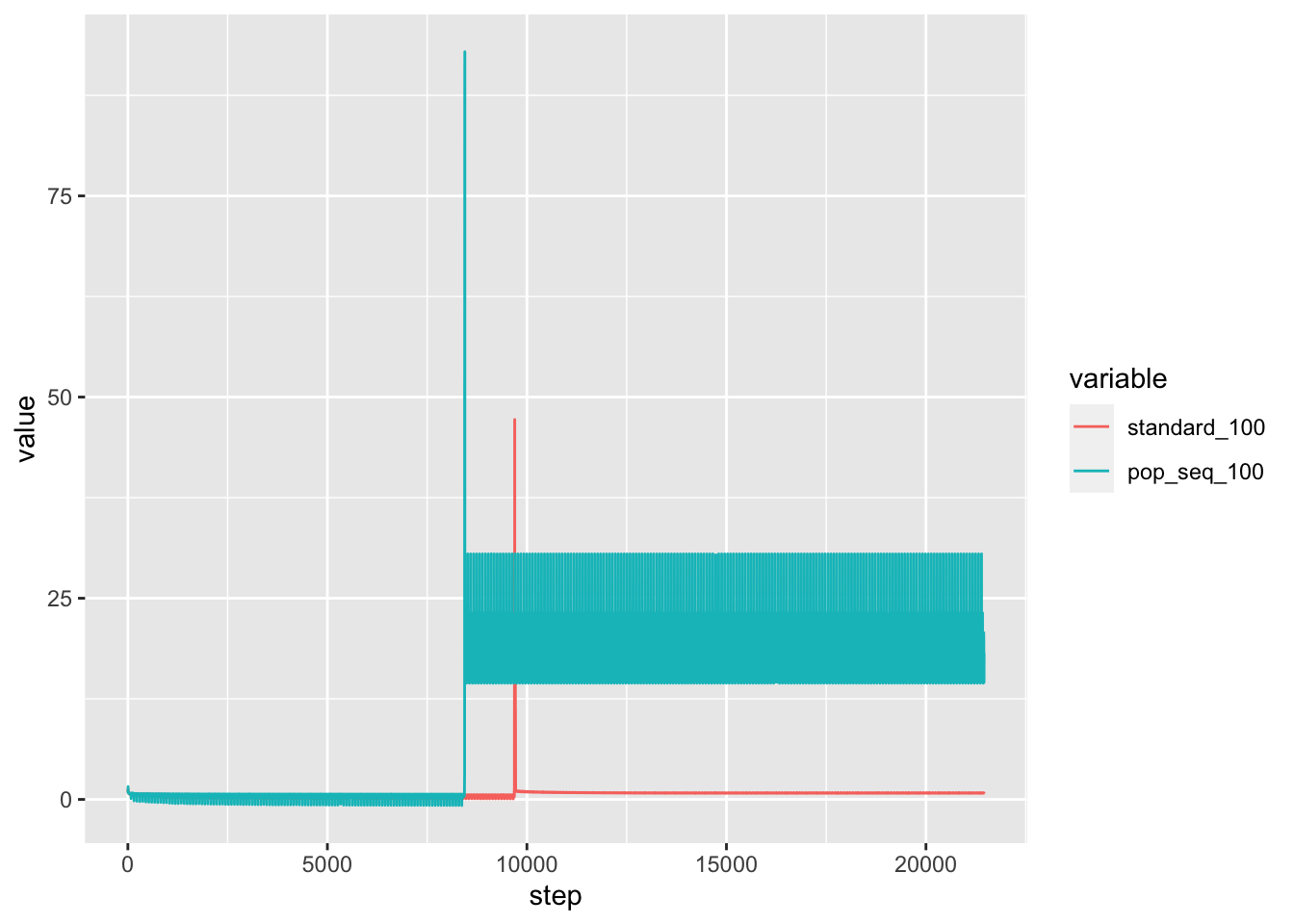
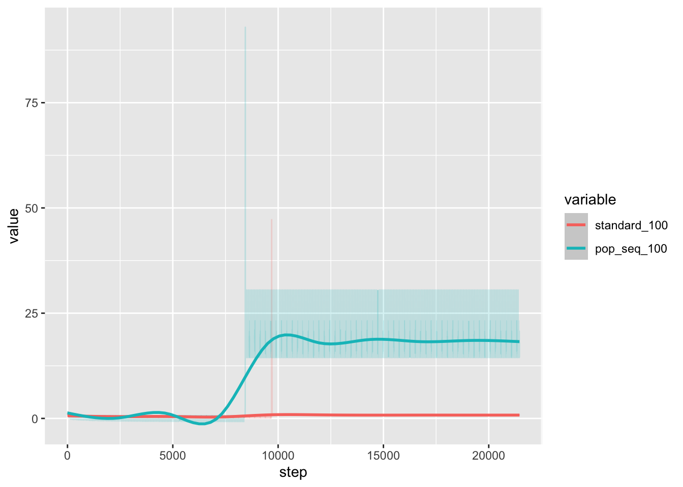
100 node training
Because I haven’t yet implemented smart restart of the training, the most “advanced” training runs so far are the 100 node training runs. I downloaded the loss data from the runs and analyze below
Because I haven’t yet implemented smart restart of the training, the most “advanced” training runs so far are the 100 node training runs. I downloaded the loss data from the runs and analyze below
Previously, I was having issues running inference and restarting training of the pytorch enformer model. This was due to issues related to saving and loading across devices (documentation here: https://pytorch.org/tutorials/recipes/recipes/save_load_across_devices.html). In a nutshell, during training the model, the model is always associated
Source Code
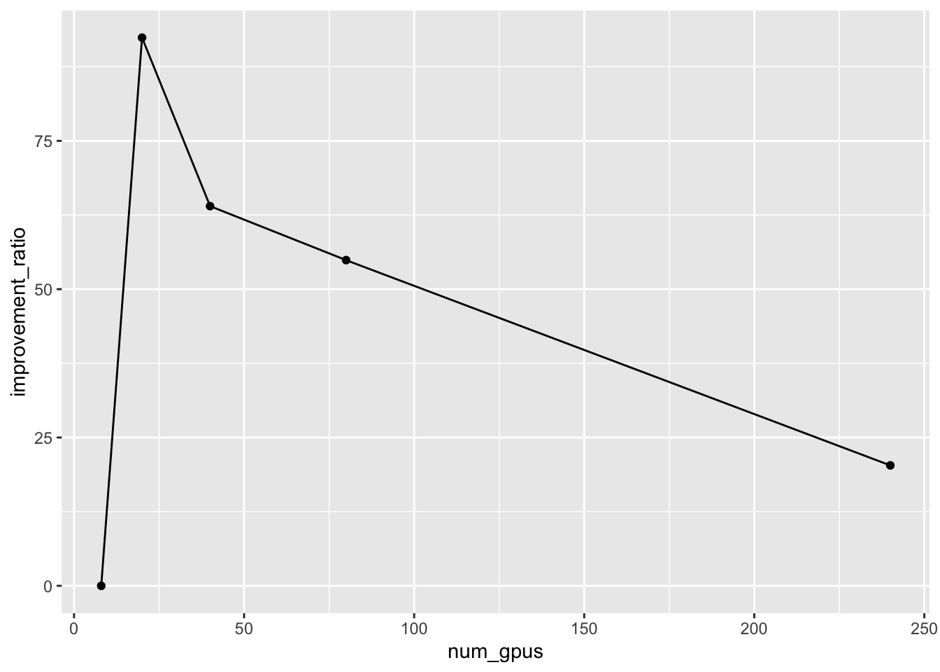
---title: "test_pop_seq_training"author: "Saideep Gona"date: "2023-06-26"format: html: code-fold: true code-summary: "Show the code"execute: freeze: true warning: false---```{r}#| label: Set up box storage directorysuppressMessages(library(tidyverse))suppressMessages(library(glue))PRE ="/Users/saideepgona/Library/CloudStorage/Box-Box/imlab-data/data-Github/Daily-Blog-Sai"## COPY THE DATE AND SLUG fields FROM THE HEADERSLUG="test_pop_seq_training"## copy the slug from the headerbDATE='2023-06-26'## copy the date from the blog's header hereDATA =glue("{PRE}/{bDATE}-{SLUG}")if(!file.exists(DATA)) system(glue::glue("mkdir {DATA}"))WORK=DATA```# ContextHave been busy working on my thesis proposal, so couldn't focus on interpreting the results of comparing the pop-seq with the standard sequences from the hackathon. Here I will begin that task## Comparing loss curves between the two training sets### 100 node trainingBecause I haven't yet implemented smart restart of the training, the most "advanced" training runs so far are the 100 node training runs. I downloaded the loss data from the runs and analyze below```{r}library(tidyverse)library(ggplot2)library(reshape2)loss_100_node <-read_csv(file.path(DATA,"100_node_loss.csv"))colnames(loss_100_node) <-c("step", "standard_100","standard_100_MIN","standard_100_MAX","pop_seq_100","pop_seq_100_MIN","pop_seq_100_MAX")loss_100_node <-melt(loss_100_node, measure.vars =c("standard_100","pop_seq_100"))loss_100_node_start <- loss_100_node %>%filter(step <100000)ggplot(loss_100_node) +geom_line(aes(x=step, y=value, color=variable))ggplot(loss_100_node_start, aes(x=step, y=value, color=variable)) +geom_line(alpha=0.2) +geom_smooth()```### 60 node trainingBecause I haven't yet implemented smart restart of the training, the most "advanced" training runs so far are the 100 node training runs. I downloaded the loss data from the runs and analyze below```{r}loss_60_node <-read_csv(file.path(DATA,"60_node_loss.csv"))colnames(loss_60_node) <-c("step", "standard_60","standard_60_MIN","standard_60_MAX","pop_seq_60","pop_seq_60_MIN","pop_seq_60_MAX")loss_60_node <-melt(loss_60_node, measure.vars =c("standard_60","pop_seq_60"))loss_60_node_start <- loss_60_node %>%filter(step <10000)ggplot(loss_60_node) +geom_line(aes(x=step, y=value, color=variable))ggplot(loss_60_node_start, aes(x=step, y=value, color=variable)) +geom_line(alpha=0.2) +geom_smooth()```### Code for parsing the training logs manuallySome of the wandb logs are buggy, and ran out of wandb storage```{python, eval=FALSE}import os,sysimport numpy as npimport pandas as pddef parse_loss(log_file, out_file):withopen(log_file) as f: lines = f.readlines() epoch = [] loss = [] step = [] tfs = [] organism = [] c=0for line in lines: p_line = line.strip().split()for i in p_line:if'train/epoch'in i: epoch.append(int(i.split('=')[1]))if'train/iter'in i: step.append(int(i.split('=')[1]))if'train/time_from_start'in i: tfs.append(float(i.split('=')[1]))if'train/human/loss'in i or'train/mouse/loss'in i: loss.append(float(i.split('=')[1])) organism.append(i.split('/')[1]) train_dict = {'loss':loss,'epoch':epoch,'step':step,'tfs':tfs,'organism':organism }print(len(loss),len(epoch),len(step),len(tfs),len(organism)) pd.DataFrame(train_dict).to_csv(out_file,index=False)log_files = ["/grand/TFXcan/imlab/users/saideep/enformer_training/pop_seq_small_DDP_20/logs/out.out","/grand/TFXcan/imlab/users/saideep/enformer_training/standard_small_DDP_20/logs/out.out"]for log_file in log_files: out_file = log_file.replace('out.out','loss.csv') parse_loss(log_file, out_file)```### 20 node training20 node training is roughly the "sweet spot" in terms of distributed training. ```{r}popseq <-read_csv(file.path(DATA,"popseq_20_DDP_loss.csv"))popseq$type <-"popseq"standard <-read_csv(file.path(DATA,"standard_20_DDP_loss.csv"))standard$type <-"standard"both <-rbind(popseq, standard)both_human <- both %>%filter(organism=="human")ggplot(both_human, aes(x=step, y=loss, color=type)) +geom_line(alpha=0.2) +geom_smooth() +ylim(c(0.1,1))ggplot(both_human, aes(x=step, y=loss, color=type)) +geom_smooth()```## Expected full training time for different configurations```{r}num_gpus <-c(8,20,40,80,240)expected_train_time <-c(317,154,80,61,21)gpu_ratio <- num_gpus/8prop_exp_train_time <- expected_train_time/gpu_ratioimprovement_ratio <- expected_train_time-prop_exp_train_timeexp_df <-data.frame(num_gpus=num_gpus,log2_num_gpus=log2(num_gpus),expected_train_time=expected_train_time, log2_training=log2(expected_train_time), log2_prop_exp_train_time =log2(prop_exp_train_time),gpu_ratio=gpu_ratio, prop_exp_train_time=prop_exp_train_time, improvement_ratio=improvement_ratio)ggplot(exp_df,aes(x=num_gpus,y=expected_train_time)) +geom_line() +geom_point() +geom_line(aes(x=num_gpus,y=prop_exp_train_time), color="red")ggplot(exp_df,aes(x=log2_num_gpus,y=log2_training)) +geom_line() +geom_point() +geom_line(aes(x=log2_num_gpus,y=log2_prop_exp_train_time), color="red")ggplot(exp_df,aes(x=num_gpus,y=improvement_ratio)) +geom_line() +geom_point()```## Running inference on saved model checkpointsPreviously, I was having issues running inference and restarting training of the pytorch enformer model. This was due to issues related to saving and loading across devices (documentation here: https://pytorch.org/tutorials/recipes/recipes/save_load_across_devices.html). In a nutshell, during training the model, the model is always associated